In the classical Image-Based visual servoing (IBVS) framework, the errors signals are directly computed from image feature extracted on the image plane. In this way, an exact 3D model of the target is not required for the servoing, and the control scheme just tries to reach a given visual pattern defined as a desired image.
However, some 3D information are still needed for a correct servoing execution: for instance, in the case of point features (the simplest 3D primitives), the current depth Z must be known in order to accurately compute the so-called interaction matrix. Usually a coarse estimation of Z (e.g., the constant value at the desired pose) may be sufficient for the servoing fulfillment, but global/exponential decoupled convergence is lost due to this approximation.
In view of this problem, we propose here a general framework able to recover online the missing 3D information needed by visual servoing schemes. The idea is to design an observer that builds upon the known dynamics of such quantities, and exploits the online measurements taken from a moving camera as a feedback signal. Under suitable assumptions of persistency of excitation, convergence of the observer can be proven and, as a consequence, asymptotic recovery of the 3D structure of the target becomes possible.
Although the proposed framework has a general validity, the physical interpretation of the persistency of excitation condition depends on the specific visual feature used for the servoing. For instance, in the case of a point feature, the observer converges if and only if the camera is moving with a nonzero linear velocity (a rotation may also be present). It is interesting to note that this kind of constraint on the camera motion, already well known in the computer vision literature on structure/motion identification, can be rigorously derived with arguments based on the nonlinear observer theory. In this sense, our attempt is to merge classical computer vision issues within the framework of nonlinear system analysis.
As an interesting extension, the same observer structure can also be used to recover the unknown focal length of a camera, by exploiting the 'dual' motions of the point feature case, i.e., zero camera translation. In this case the estimation task is easier w.r.t. 3D quantities because the focal length is an unknown but constant parameter.
Documents
The observation framework has been developed by A. De Luca, G. Oriolo and P. Robuffo Giordano and published on the following papers in chronological order:
On-Line Estimation of Feature Depth for Image-Based Visual Servoing Schemes, ICRA, 2007
Image-based visual servoing schemes for nonholonomic mobile manipulators, Robotica, 2007 (see also this page)
Feature Depth Observation for Image-based Visual Servoing: Theory and Experiments, The International Journal of Robotics Research, 2008
Visual Servoing with Exploitation of Redundancy: An Experimental Study, ICRA, 2008 (see also this page)
3D Structure Identification from Image Moments, ICRA, 2008
| Matlab simulation | |||||||
|
On the left two plots of a matlab simulation are reported. In this case the observer is asked to estimate the unknown initial depth of a static point feature (set at 0.5 m away from the image plane) while the camera performs a complex rototranslation motion. The initial depth state of the observer is set at 1.0 m. On the left picture the feature/depth error are shown, while on the right picture the behavior of true and estimated Z is reported. Note how the estimated value quickly approaches the true value despite of a complex camera motion. |
|
||||||
| Webots simulation | |||||||
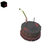
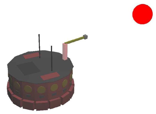
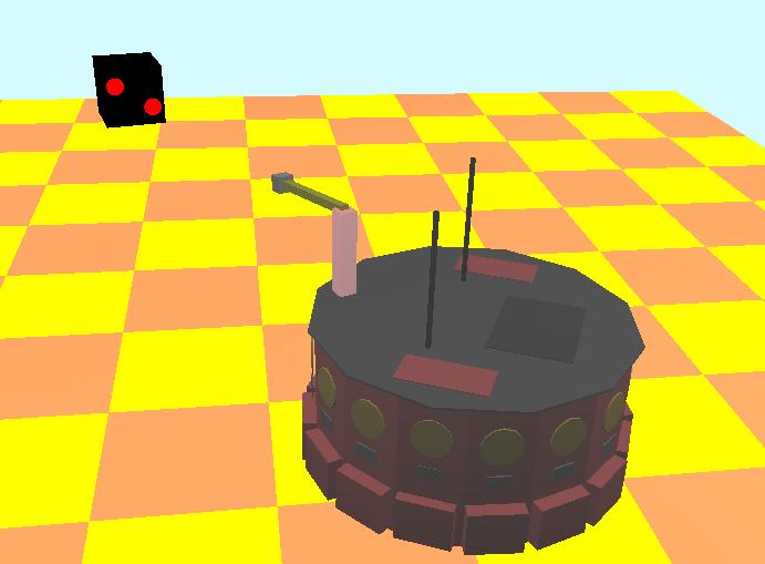
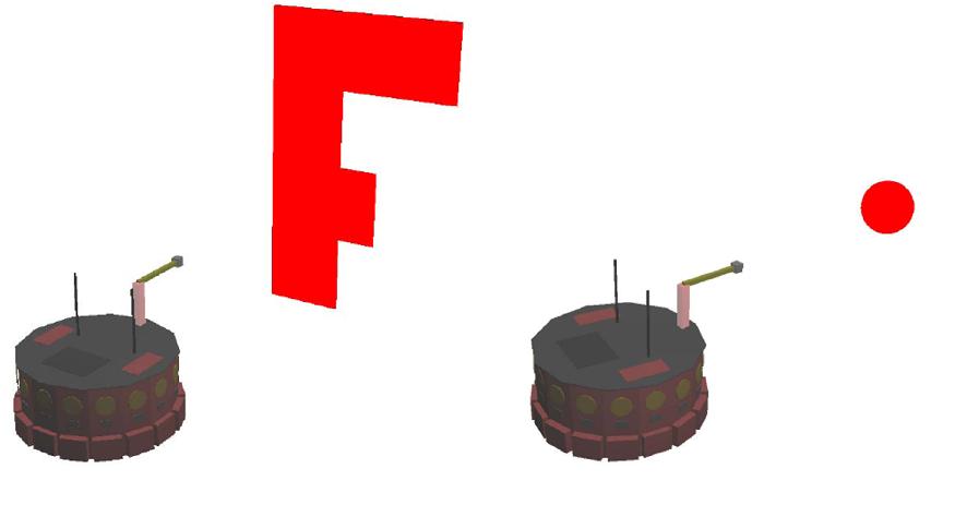
In this second simulation, the observer is tested in a more realistic environment, i.e., within a 3D simulated world (Webots) where a
nonholonomic mobile manipulator (NMM) with a camera on the end-effector tracks the red dot on the cubic target. The presence of noise
on the extracted image coordinates does not prevent the estimation convergence, as it can be checked in the two pictures on the right. |
|
||||||
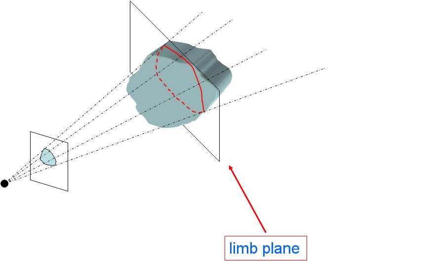
Sometimes tracking and matching individual structures during the camera motion, i.e., solving the so-called correspondence problem, is not easy or convenient (think to dense objects as spheres, ellipsoids, etc.). When this is the case, IBVS schemes usually rely on more global (integral) features, like image moments, instead of local descriptors like feature points. Indeed, moments can be directly evaluated on any arbitrary shape on the image plane and are free of the correspondence problem that typically affects the identification of common geometric structures. Of course, these nice properties come at a price: when considering moments, the 3D information present in the relative interaction matrix does not reduce to a simple punctual depth, but more general 3D structures are involved. To understand this fact, consider the figure on the right. One can associate to most 3D shapes a special plane, called limb plane, made of all those 3D points whose projection traces the shape contour on the image plane. It can be shown that the 3D information needed by the interaction matrix of a generic moment is the unit normal vector of the limb plane scaled by its distance from the camera optical center. As in the point feature case, it is possible to extend our observation scheme also to this case, and recover online the missing 3D information. |
 |
| Webots simulation | |||||||
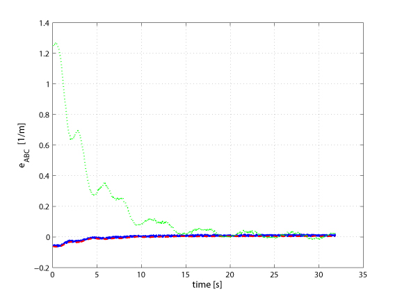
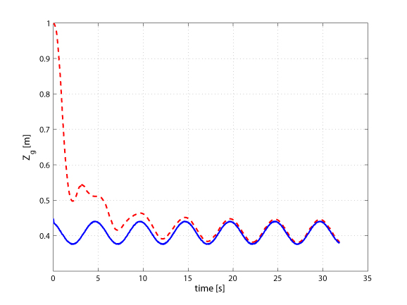
In this simulation, we tested again the observer in the Webots environment. The moments used for the estimation are the area a and the barycenter (xg, yg) measured from the projection of a sphere with radius R=0.07 [m] and lying at a distance of about 0.4 [m] from the camera. As before, the robot is commanded with a predefined periodic motion to provide the needed camera mobility. The left picture shows the error in estimating the three components of the scaled normal vector, i.e., all the information needed by the interaction matrix. By exploiting the estimated distance of the limb plane, it is also possible to recover other 3D information like the depth of the center of the sphere, as shown in the right picture. |
|
||||||
| Robot and target object | |||||
|
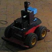
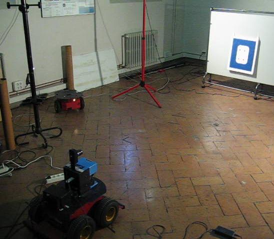
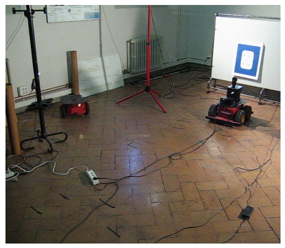
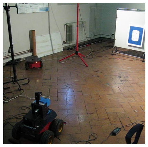
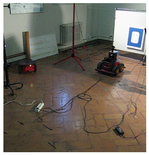
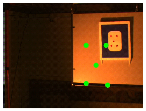
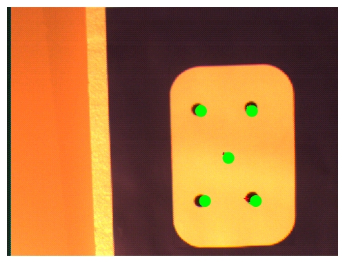
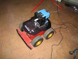
In our experiments, we used a unicycle-like robot equipped with a fixed camera mounted on its top. This design can be seen as a particular case of the more general class of standard manipulator arms mounted on a nonholonomic mobile platform, thus realizing a nonholonomic mobile manipulator (NMM). More details on kinematic modeling and control for NMMs can be found here, while in this page the specific case of IBVS tasks for NMMs is discussed. As for the target to be tracked, we chose a vertical planar object with 4 black dots placed at the vertexes of a rectangular shape. |
|
||||
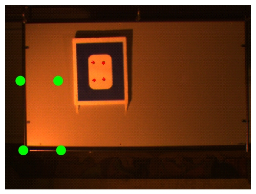
| Servoing with point features | |||||||||||
|
| ||||||||||
| Servoing with image moments | |||||||||||
|
|
||||||||||
| Estimation of the focal length | |||||
In this last experiment, the goal was to estimate the focal length of the camera
while the robot was tracking a feature point during its motion. This estimation was performed by using an extension of the proposed observer as discussed at the beginning of the page. We wish to thank Prof. Prattichizzo and his team for their support to our experiments. |
|
||||
Video
|
We propose a sample video representative of all the experiments. Note how, at the beginning, the servoing is not converging, i.e., the feature points are not approaching the desired positions. This is a direct effect of the intial wrong depth estimation. After some seconds, however, the observer converges and a proper image plane feature trajectory is recovered, allowing the realization of the visual task. |